Outperforming cuBLAS on H100: a Worklog

CUDA matmul kernel - from scratch

In this post, we’ll iteratively implement a CUDA kernel for matrix multiplication on latest generation¹ NVIDIA hardware: H100.

We’ll gain a deep understanding of H100 architecture and showcase these optimizations step by step. The final kernel outperforms cuBLAS by 7% for N=4096. It fits in a single C++ file without any dependencies.

This post is intended as a sequel to Simon’s legendary blog which showcases similar optimizations for A6000 GPU. However H100 GPUs are completely different beasts, requiring entirely different algorithms. As an example, algorithm from Simon’s blog is only able to achieve 4% of cuBLAS performance². In this post, we will pick up from Simon’s blog and iteratively reach 107% of cuBLAS.

All my code is available on Github.

Our aim is not to be a cuBLAS replacement, but to design a slightly faster, yet simplistic, matmul kernel which works for generally large matrices. cuBLAS performs well for varying matrix sizes, like small matrices with very large k-dimension or matrix-vector multiplications(relevant for LLM inference).

Quick recap from Simon’s blog

Let’s go over basic structure of matrix multiplication algorithm that Simon covered. We compute C[m, n] = A[m, k] x B[k, n] as shown in figure below:

This image is not mine, and taken from Simon’s blog

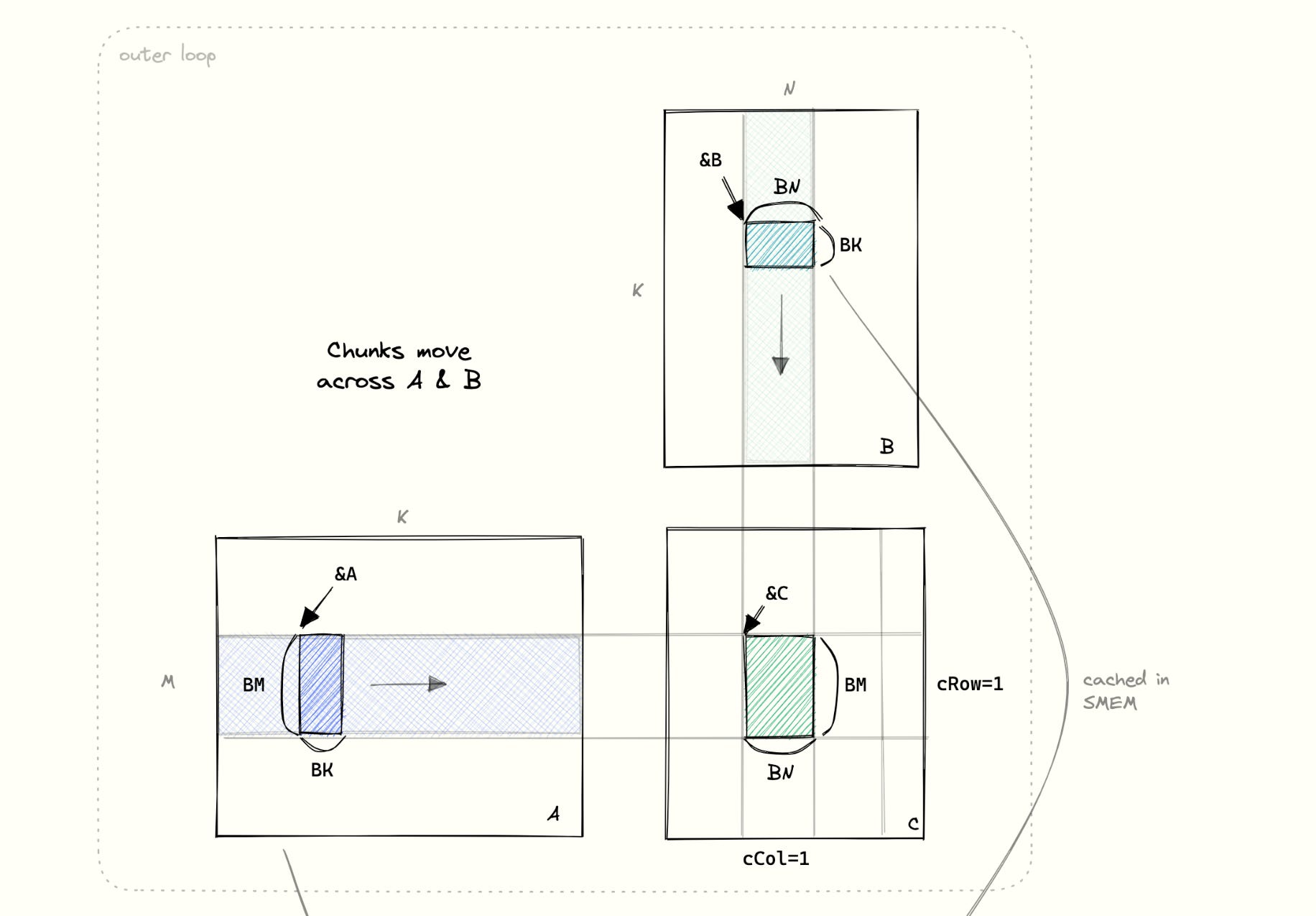
We break down large matrix multiplication into computing several output tiles. Each tile is BM x BN size - which represents a portion of output matrix C. We assign a thread block to compute this tile - which has upto 1024 threads working together.

To compute all outputs in this tile. we will need to read BM x K row-block from A(blue) and K x BN column-block from B(green). These values are accessed multiple times, so we need to store them in SMEM for performance.

However, these blocks are too big to store in SMEM. So we store them in chunks of BK size. For each chunk, we can multiply BM x BK and BK x BN matrices and get a BM x BN matrix for output tile. Remember the naive matrix multiplication:

As the chunks are in k-dimension, we simply need to sum all these matrices to compute final values of BM x BN output tile. All the values in output tile are stored in registers, so accumulations are easy.

Our H100 matmul kernel will follow this structure of computing output tiles by multiplying smaller chunks of matrices. Simon’s blog goes on further to fully utilize register space by moving parts of chunks from SMEM to registers. We will not go over these details here, as we don’t use them in our kernels.

Setup

For rest of the blog, we will consider large matrices of square sizes (M=N=K=4096) with bfloat16 types. bfloat16 is a specialized 16-bit data type used in recent deep learning applications. For our kernel performance, it isn’t any different from regular fp16. Matrices B and C are stored in column-major, while A is stored in row-major. This is a common setup for matmul benchmarks.

We initialize our matrices using a normal distribution with mean = 0 and std_dev = 1. It turns out this is the best distribution for performance measurement. Interested readers can refer to this blog from

Horace He

for more details.

For measuring flops, we average running time over 8 runs(ignoring the first warmup run). Then FLOPS are calculated by 2 * m * n * k / time.

All benchmarks are run on H100 SXM with CUDA toolkit 12.6, V12.6.68

What lies in H100

Let’s go over some H100 specifications to understand new characterstics of this GPU.
H100 comes in two variants: PCIe and SXM. They are very similar, except that the SXM variant is slightly faster. My machine has H100 SXM, which has the following specs:

• 132 Streaming Multiprocessors(SM)

• 1024 threads per SM

• 4 Tensor Cores per SM

• 80GB High Bandwidth Memory (3.35TB/s)

• 256KB combined Shared Memory + L1 cache per SM

• 65,536 registers per SM

• 50MB L2 Cache shared between all SMs³

Most of these terms are familiar from the previous blog. Compared to previous generations, H100 GPU has more SMs, faster global memory, faster clock speed, more shared memory and larger+faster L2 cache. Matmul kernels use all of these features - so we can expect an old-gen algorithm to naturally perform faster on H100. We indeed see a jump from 21 TFLOPs on A100 → 32 TFLOPs on H100.

We clearly have a long way to get close to cuBLAS (716 TFLOPs). The key lies in a new spec that we haven’t seen before:

Tensor Core

Tensor core is a special hardware unit in GPU which does small matrix-matrix multiplications in a single hardware instruction. This comes in multiple flavors - mma wmma and wgmma instructions.⁴ In this blog we’ll look at the wgmma instructions which are introduced by Hopper architecture.

Unfortunately, there’s no documentation of these instructions in CUDA C++ guide and we have to look at PTX guide. (yes we’ll have to write these assembly-like instructions in PTX instead of C++). Let’s look at an example instruction:

wgmma.mma_async.sync.aligned.m64n16k16.f32.bf16.bf16

This executes a matrix-multiply operation C = A*B + C with m=64, n=16 and k=16.

• A: mxk matrix of bfloat16 type stored in shared memory.

• B: kxn matrix of bfloat16 type stored in shared memory.

• C: mxn matrix of 32-bit float type stored in registers.

Storing A and B needs (64*16 + 16*16) * 2 bytes = 2.5KB shared memory.

Storing C will need 64*16 = 1024 registers.

Note that a single gpu thread can only store upto 256 registers - hence tensor core instructions require storing C over 128 threads in a SM! Note that a warp = 32 threads, so 128 threads will comprise 4 warps. A group of 4 warps is called a warp-group in Hopper architecture. When we distribute C over a warp-group, each thread needs 1024/128 = 8 registers - which is a much resonable number. Note that the instruction is called wgmma which stands for warp-group-matrix-multiply-add.

Asynchrony

Note the term mma_async in tensor core instructions. These instructions are run asynchronously on the 4 tensor cores per SM. Consecutive tensor core instructions can be batched together and sent to tensor cores, running them in parallel. This is vital to fully utilizing all tensor cores. Full PTX code for these instructions is a bit verbose. We go over the details in Appendix section. Throughout the blog, we will use them like this:

Instruction sizes

H100 offers several such matrix multiplications instructions of varying sizes. From PTX guide:

.shape   = {.m64n8k16, .m64n16k16, .m64n24k16, .m64n32k16,
                                 ...
                                 ...
            .m64n232k16, .m64n240k16, .m64n248k16, .m64n256k16};

Among all these instructions m=64 and k=16 remain the same. n can vary from 8 → 256. Based on my experience, it is faster to use a single instruction with larger n, than multiple instructions with smaller n. However, note that larger n uses more resources. n=256 demands a whopping 40KB of SMEM and 128 registers per thread!

Kernel 1: Simon’s blog

Simon’s algorithm was designed for FP32 types. Adapting it for bfloat16 types gives us 32 TFLOPs.

Note that this is not a fair comparison, as cuBLAS leverages tensor core operations for bfloat16 which are unavailable for FP32. In the blog post, Simon claims this can increase performance by 3.5x, but couldn’t get to it. We will pick up where he left off, and start using them.

Kernel 2: Using Tensor Core instructions

We are now ready to write a simple kernel which computes output tile using tensor core instructions. This section is a bit lengthier than I wanted, but it sets up the core concepts that we need through rest of the kernels.

We will assign one output tile to each thread block, which will have 128 threads cooperating to execute a tensor core instruction. This is very similar to Kernel 5 from Simon’s blog. We will simply replace hand-written matrix multiplication of blocktile with a tensor core instruction.

Let’s use WGMMA_M=64, WGMMA_N=64, WGMMA_K=16 notation to denote sizes of wgmma operation. For simplicity, let’s match our block size with wgmma size making our kernel simpler. Here’s the overall kernel structure:

Note that we follow the same kernel structure previously discussed:

• We loop over K-dimension in chunks of size BK. For each chunk:

  • We load corresponding chunks from A and B into SMEM

  • We use a tensor core instruction to multiply these chunks and store them in registers

• After all chunks are processed, we write values in registers to corresponding tile in C.

Note that we have skipped the code to load and store chunks. Let’s go over the loads first.

Tensor core instructions need a very specific layout of chunks in SMEM - which isn’t simply row or column major. Here’s the diagram from Nvidia:

This layout is heavily swizzled and too complex to be loaded by hand. Nvidia has implemented swizzling is order to avoid shared memory bank conflicts. Moreover, the memory layouts in diagram are incorrectly documented. Thankfully, Nvidia provides an out-of-box way to load tiles without worrying about these layouts: Tensor Memory Accelator(TMA).

Loads using Tensor Memory Accelerator (TMA)

TMA is a new hardware piece introduced in Hopper architecture. It is a faster way to load tiles of multi-dimensional matrices between GMEM and SMEM. This is implemented in an independent hardware unit, making it much faster than custom loads. TMA loads directly support the swizzling patterns required by tensor cores.

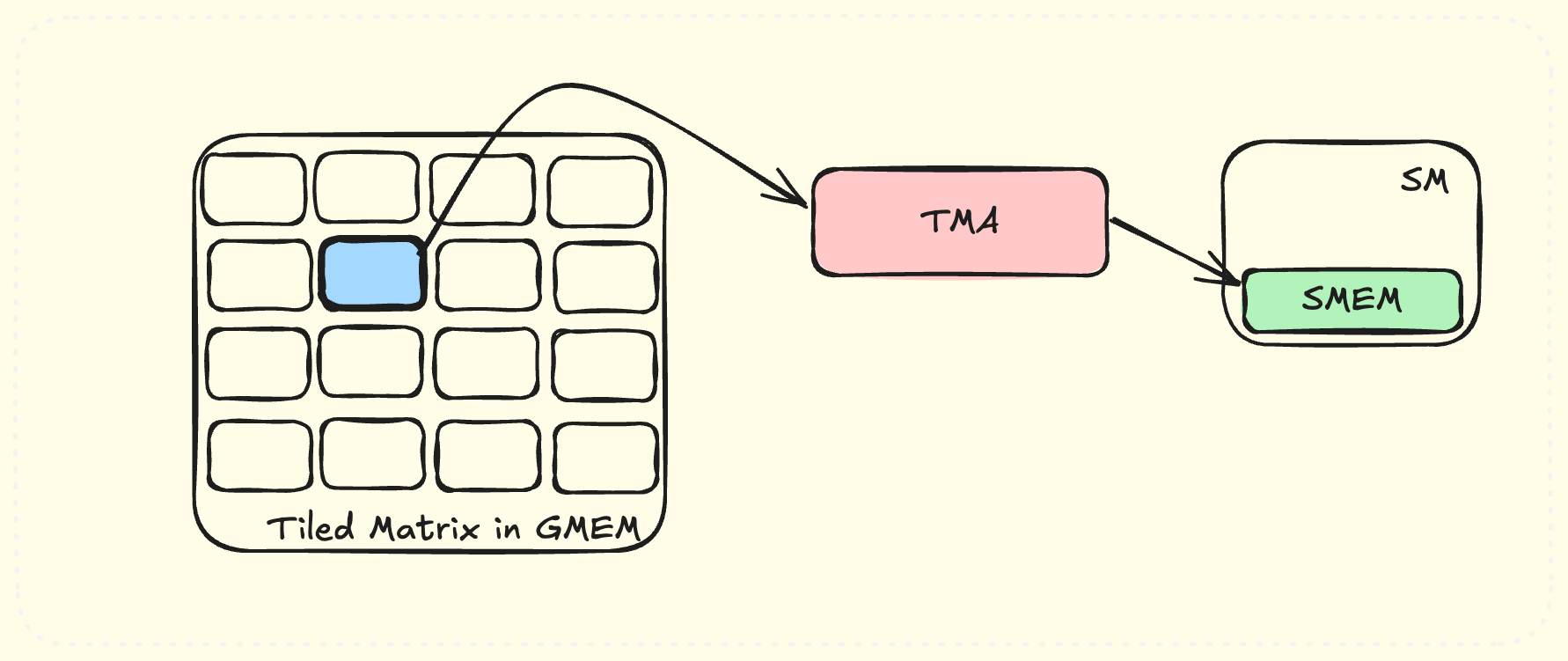
TMA takes in a tiling configuration of matrix, and can load any requested tile into SMEM.

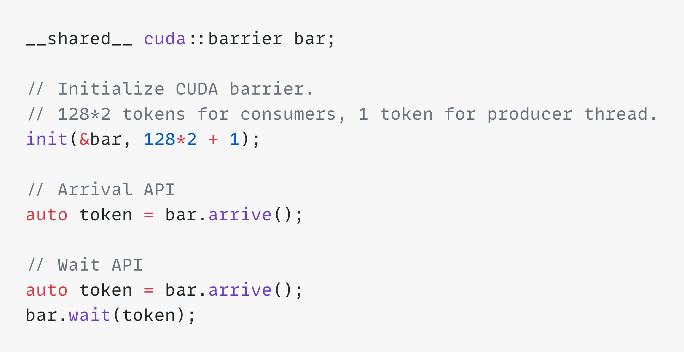
One difference with TMA loads is that it needs to be called from a single thread. Previously, multiple CUDA threads cooperated to load a chunk of memory. Using TMA, a single thread can issue a TMA call, and all threads wait for it to finish. Following example, taken from CUDA programming guide, can be used to load a tile of A into SMEM. It uses cuda barriers to wait for the loads to finish:

Storing output tile

Values of output tile are stored across 128 threads in a thread block. It is possible to compute the mapping from thread id, register index → corresponding global memory address:

(threadIdx, registerIdx) → (idx in BM x BN tile)

Once we have the mapping, we can store all register values to GMEM. There’s nothing special about the mapping function, and I don’t recommend readers diving into it. We should just realize its a simple arithmetic mapping that can be computed when we want to:

Performance

We reach 317 TFLOPs throughput, a big jump over 32 TFLOPS of previous kernel. We also introduced several new features in this section: Tensor cores, TMA and CUDA barriers. All of these work together to give us a nice 10x boost in performance!

Tensor cores indeed pack a lot of power. Note that A6000 gpu also has tensor cores, but it’s possible to achieve 92% throughput without using same. This is not true for H100, where tensor cores are mandatory for high throughput.

We will keep improving our kernel using these features and more new H100 features in following sections :)

Kernel 3: Handling larger output tiles

We have previously set tile size equal to tensor core instruction. However, it is also possible to use larger values of BM and BN. We just need to break down this matmul into smaller matmuls as we’ve done before. We simply loop over M, N, K dimensions and perform a regular matrix multiplication of size [BM/WGMMA_M, BK/WGMMA_K] * [BK/WGMMA_K, BN/WGMMA_N] :

Performance

This reaches performance of 423 TFLOPs with BM=128, BN=128, BK=64 and using m64n128k16 wgmma instruction. Note that tensor cores provide a range of instructions for different values of n. It is always better to use the largest available instruction and set BN = WGMMA_N.

Profiling

Our kernel does 3 basic things during its lifetime: Loads, Tensor Core operations, Stores. Loads and TC operations are done in a loop over k-dimension. Once the computation is finished, we Store all values to output matrix:

This visualization is important to uncover further optimizations. First, let’s also quantify our visualization and measure how much time each load/compute/store phases take. This is measured in number of clock cycles spent by GPU thread:

Once we have times spent for all operations, we can store this information in a global array at the end of kernel:

Once kernel has finished running, we will average load time taken for all thread blocks. Note that storing information for one thread from each thread block is enough for our usecase. Here’s what we find:

Load: 1415
Tensor Core: 703
Store: 4572

We see that tensor core operations are 2x faster than loads. Store operation is 6.4x slower, but only runs once compared to Load+Tensor Core loop which runs 128 times. These numbers change with different tile sizes, but quantifying them gives us a good picture what’s happening.

Kernel 4: Hiding load latencies

Interestingly, it is possible to hide the load latencies if we run loads and tensor core operations in parallel.

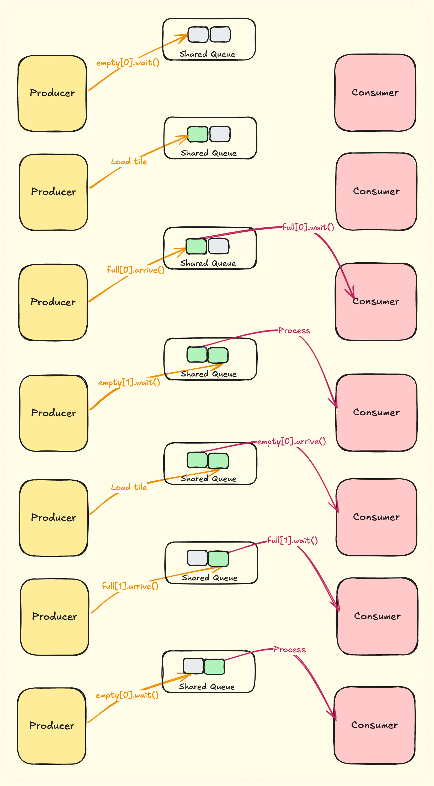
Think of this as a producer-consumer problem. We run tight loops of Producer(loads) + Consumer(tensor cores). Instead of running them sequentially, let’s decouple them and run them in parallel.

Producer will keep loading chunks and keep putting them in the queue. Consumer will keep dequeueing items as they arrive and process them. A queue can also store multiple items if producer is fast enough to produce them. This way, both producers and consumers are not affected by each other’s latencies.

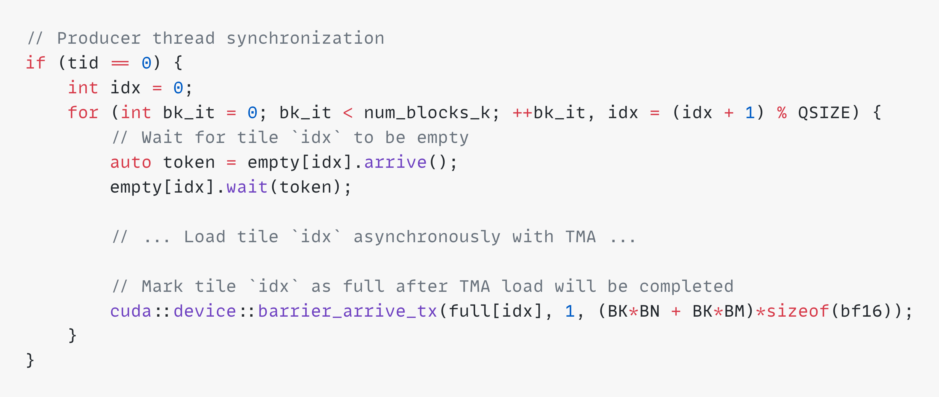
To implement this, we will use the “Warp Specialization” technique from CUDA programming guide. This starts 2 warpgroups in a thread block. One warpgroup acts as a producer and other as a consumer. We will use barriers and a circular buffer to implement shared queue.

Let’s initialize our data structures:

Producer will keep loading tiles into shared buffer starting from index 0 in a circular way. Before loading tile, it calls empty[i].wait()to check if the index in shared buffer is ready to be filled. After filling the index, it calls full[i].arrive()to signal the producer that this is ready to be consumed.

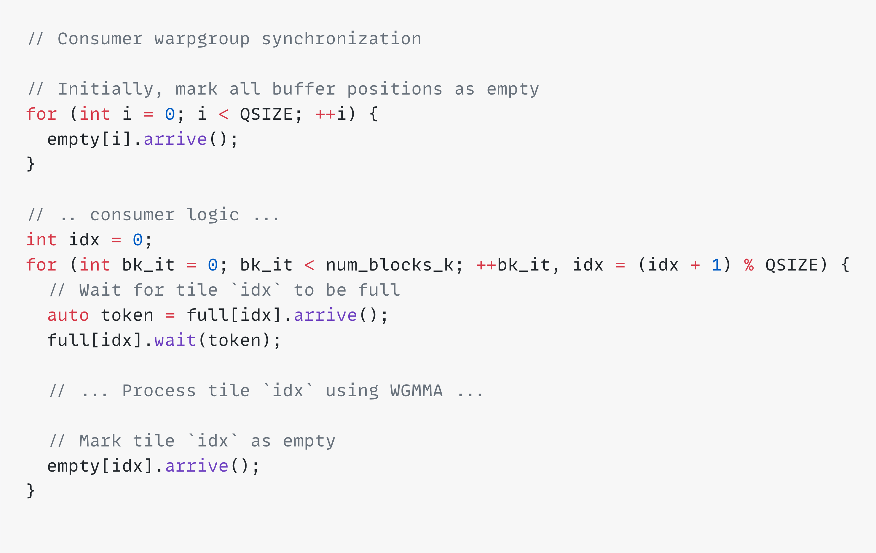
Similarly, consumer calls full[i].wait()to wait till tile is loaded into the index in shared buffer. After consuming it, it signals producer by calling empty[i].arrive(). Note that we initialize our barriers in a way that producers think the shared buffer is empty at the very beginning.

Here’s is a flow diagram with a shared buffer of size 2. We show the state of queue after each interaction with producer/consumer. Note that both producer and consumer run in parallel, and their speeds may not be same as this example:

Performance

This reaches performance of 498 TFLOPs with 128 x 128 tile sizes and QSIZE=5.

Kernel 5: Pushing Tile size limit

So far, we have been using tile sizes of 128 x 128. Let’s see if we can push this to 128 x 256. This will allow us to use a larger wgmma instruction, and also reuse memory loads.

Limiting factors for larger tile sizes are: SMEM size and register size. Let’s try increasing the tile size and see what happens:

ptxas info : (C7511) Potential Performance Loss: wgmma.mma_async instructions are serialized due to insufficient register resources for the wgmma pipeline in the function 

'_ZN2M413matmulKernel4ILi128ELi256ELi64ELi256ELi3ELb0EEEviiiP13__nv_bfloat16PK14CUtensorMap_stS5_Pi' 

Performance: 123 TFLOPs

We see a compiler warning of “insufficient register resources”, and a 5x dip in performance. Output tile uses 128 x 256 = 32768 registers in the thread block, which is only 50% of total register usage. This leaves more than enough room for other registers used by kernel to store variables. Clearly this isn’t the problem. Let’s look at register usage per thread instead:

For 128 x 256 tile size, we will need 256 output registers in a warpgroup of 128 threads. 256 is already the maximum limit of registers a thread can have on H100. On top of this, the kernel will use more registers to store the variables as well. When a thread hits limit of register usage, it will store some registers to memory when they are not needed and load them back later when needed. This is called register spilling and considerably slows our kernel. In our case, spilling is done between tensor core operations, due to which they are serialized, and cannot be batched.

Using 2 consumer warpgroups

We know that we hit per-thread register limits, but not the overall register limits in a SM. The solution is simple, just use more threads! We will use 2 warpgroups to work together and do the wgmma operations. After loading the tile, we split the tile into two 64 x 256 tiles, and 2 warpgroups can compute output of each tile. Per-thread register usage will be halved while keeping the overall register usage same.

This is surprisingly simple to implement. We simply need to start a kernel with 128*3 threads. We will have 3 warpgroups: One producer and Two consumers. Note that while the consumers process the output tiles in parallel, but they still wait for the whole chunks to be loaded by the producer. Both consumers will use the same code, except processing different parts of loaded tiles. They arrive and wait on same barriers at similar times. We just need to initialize barriers with higher token counts:

Performance

This gives us a nice boost in performance to 610 TFLOPs. Larger tile size is also more SMEM hungry - making us reduce QSIZE from 5 → 3. However, we still see an overall performance boost.

Profiling shows that each thread uses 168 registers. Total register usage in a thread block of 3 warpgroups sums to 64512, which is just under the GPU limit of 65536 registers. Note that while consumer warpgroups need the high register usage, producer threads don’t need to use these many registers, as they don’t perform tensor core operations. Typically, nvidia compiler assigns same number of registers to every thread. However, Hopper architecture allows us a way to specify per-thread register usage of a warpgroup using PTX:

Using these values still keeps our register usage to 64512 (240*128*2 + 24*128), but shifts register usage from producers to consumers. This boost performance up to 631 TFLOPS.

This performance boost is nice to have, but hard to reason about. My theory is larger register count in consumers leads to fewer register bank conflicts. Please let me know in comments if you have other explanations!

Kernel 6: Hiding store latencies

We were able to hide load latencies by separating producers and consumers. Let’s see how we can hide store latencies.

A SM processes multiple output tiles throughout the kernel lifespan. For first tile, we see that loads and tensor core operations are parallelized. At the end, we store all computed values to C matrix. During this time, we can also start loading chunks for the next output tile. Note that store and load operations do not use any common resources. Loads are stored in SMEM, while stores are done from RMEM to GMEM.

According to our profiling, around 4572 cycles are spent in storing values to GMEM. If we start loading chunks for next thread block during this time, we can load 4572 / 1415 = 3.2 chunks. This means, consumers for next thread block can start running immediately after finishing current thread block!

To implement this, we start our kernel with as many thread blocks as SMs - 132 for H100.

Now, we need to decide which tiles are assigned to which SM. Previously, we had 1 tile for each thread block, and we let the GPU schedule these on different SMs. Now, we need to do this scheduling by ourselves. Let’s follow a simple scheduling logic of assigning consecutive output tiles to a SM:

We don’t need much additional logic to overlap stores and loads across tiles. When processing a new tile, we will be reusing the barriers and shared queue instead of re-initializing them. Once the producer finishes loading chunks for a tile, it will immediately start loading chunks for next tile. Consumers will also know when they have finished processing a tile, and can start reading from next position in shared queue for next tile.

Performance

We see 400 TFLOPs with this strategy, which is a regression from previously 640 TFLOPS! That did not work as well as we planned. Our overlapping stores logic is pretty sound, let’s see if we have messed up with our scheduling logic.

Scheduling and L2 Cache

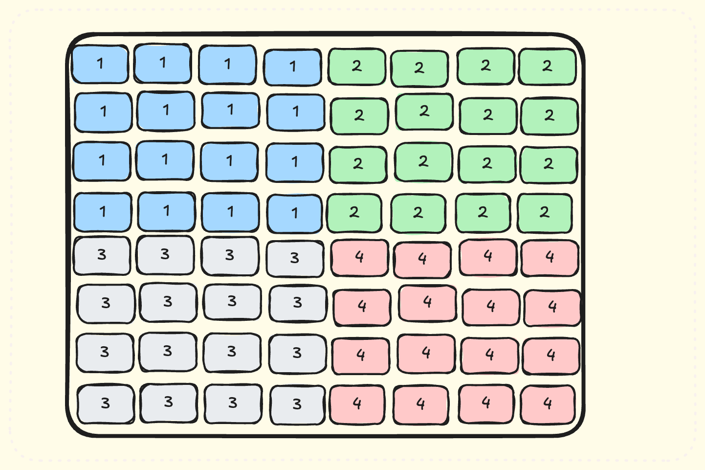
Instead of looking at what tiles are processed by a single SM, let’s look at the first tile processed by SMs. These tiles will be processed at the same time.

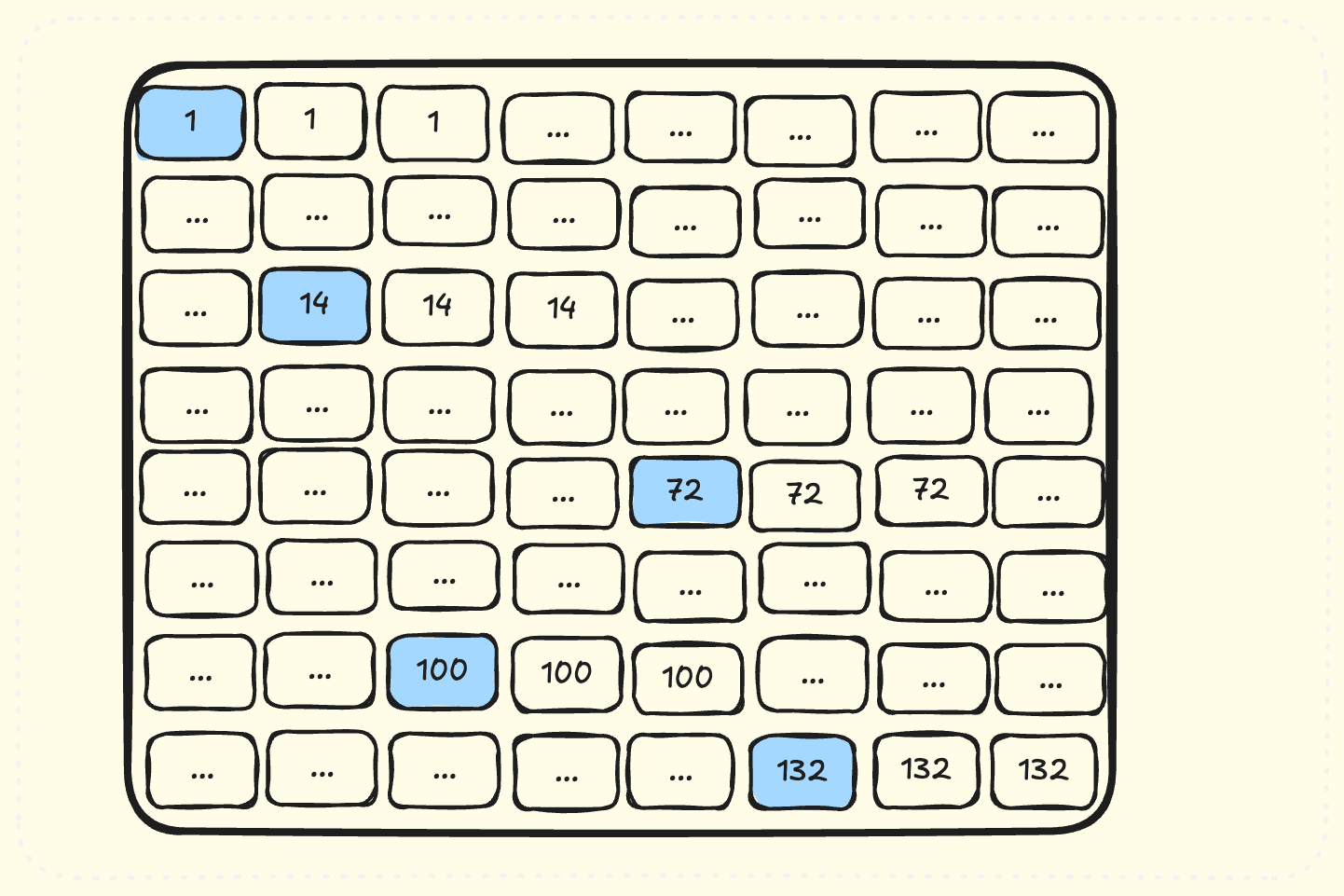
We see that SMs process very far-away tiles at the same time. This means loading very different chunks of memories from A and B matrices at same time. If we are able to schedule nearby tiles at same time, then their loaded values will have lots of common parts of A and B matrices. These common parts will be cached in L2 cache of GPU - meaning we don’t have to load tiles from GMEM all the time! Let’s see how this scheduling looks like:

Diagram not to scale, 4 x 4 regions correspond to 128 tiles (16 x 8)

Note that same colored tiles are scheduled at same time. This means lots of common accesses to A/B matrices at same time - all served by L2 cache!

Note that we used only 128 SMs in the diagram because it is easily groupable in 16 x 8 configuration. Making everything a power of two makes our scheduling logic much simpler.

Performance

660 TFLOPs. We hit a L2 cache hit rate of 83%, meanwhile cuBLAS only hits 70% L2 cache hit rate.

It is not hard to modify the logic to use all 132 SMs. We can still keep this configuration but assign some tiles in next group to leftover SMs. We keep doing this till we go over all tile groups. Also, our tile configuration need not be 16x8, it can be something small like 2x2 as well.

After trying several tile group configurations, I found that using 132 SMs instead of 128 SMs is slower(655 TFLOPs). This is because our tile counts divide roundly into 16 x 8 regions - leading to better L2 cache hits if we use 128 SMs.

Kernel 7: Faster barriers

Note that our current barrier implementation is recommended by the CUDA programming guide. It turns out there exists a faster barrier implementation which can significantly speed up our kernel. This implementation is only referenced in the PTX guide, without any CUDA API. And it is left as an exercise to the reader as to which one is better :)

Let’s list out both barrier APIs, and start using the new one!

CUDA Barrier API

PTX Barrier API

There are 2 differences in the APIs:

• Phase variable: We manually keep track of phase variable, which is parity of how many times we have called wait on the barrier. There is no other significance to the phase variable. The underlying API demands we manually track this and pass this in the API. This is an abstraction leak, which is probably needed for performance reasons.

  • Note that we do not need to re-initialize a barrier once the wait call has completed. We can simply reuse it as it was freshly initialized with previous values. A barrier is typically reused hundreds of times as we load hundreds of tiles in shared queue.

• Tokens: Another difference is that this API does not use any tokens in arrive and wait calls. This makes the implementation cleaner, and allows us to further optimize our synchronizations. This means that not all threads who execute wait need to have called arrive first. We can reduce number of token synchronizations to from 257 to 3(one per producer and consumer). Using less synchronizations makes our code faster:

Note that the new API needs to be implemented in PTX. These are simple CUDA wrappers over PTX code, highlighted in the github code.

Performance

The new barrier API gives a nice 10% performance boost, getting us to 704 TFLOPs. We have now achieved 98% performance of cuBLAS. The remaining optimizations will give us smaller returns, but will slowly take us upto and further than cuBLAS.

Kernel 8: Thread Block Clusters

Clusters are a new Hopper feature which groups multiple thread blocks running concurrently across multiple SMs. Multiple SMs in a cluster can synchronize and collaboratively fetch and exchange data.

To use this feature, we need to declare this in the kernel function definition:

// This launches a kernel with 2 SMs in each cluster.

__global__ void  __cluster_dims__(2, 1, 1) kernel(...) {
  // ... kernel code
}

TMA Multicast

Multiple SMs in a cluster can load the same tile using TMA multicast operation. This is faster than loading the tile twice from L2 cache. Nearby tiles read same chunks from input matrices, making this feature very useful.

Above figure shows when 2 vertically consecutive tiles run on different SMs in same cluster. They need to load 2 different chunks from A, but same chunk from B. This chunk from B can be multicasted to the SMs in the cluster. TMA supports this functioanlity.

TMA multicast operation is a PTX instruction. Like other cases, this is not complex, but lacks a wrapper function in CUDA.

cp.async.bulk.tensor.2d.shared::cluster.global.tile.mbarrier::complete_tx::bytes.multicast::cluster

In order to use this, we will also need to synchronize barriers across different SMs in a cluster. PTX barrier provides this functionality by appending cluster keyword to the arrive function. We provide wrappers to both methods in our github code.

Performance

This gets us to 734 TFLOPs. We are now doing slightly better than cuBLAS, at 102% of cuBLAS performance.

Note that it is possible to group cluster in different ways(horizontal tiles), and even using cluster of size 4 with 2x2 tiles clustered together. Our implementation supports all cluster shapes, but we found vertical clustering of 2 tiles to be the fastest. This compensates our uneven tile size(128 x 256). Using larger cluster sizes is much slower, likely due to expensive inter-SM synchronization.

Kernel 9: Micro-optimizations

This kernel includes a series of small optimizations.

• Reordering stores:

  • We write values of several registers to GMEM. We can order them in a way that consecutive writes map to nearby memory locations. This results in slightly better performance. Relevant part of our store logic:

    

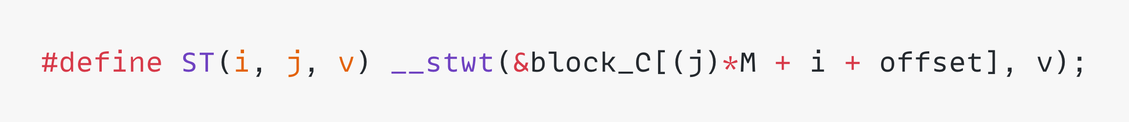
• Skipping L1/L2 cache for writes:

  • We can use cache hints to skip store the value directly to GMEM, skipping L1/L2 caches - freeing up slightly more space for A,B matrices. Using __stwt() method provided by CUDA:

    

• Skip resetting registers to 0:

  • Remember that Tensor core operations accumulate values, therefore we need to reset their registers to 0 between processing different tiles.

    

  • If we look into tensor core spec, it is possible to set a flag to control whether tensor core operation does the accumulation. This switches the tensor core operations between C = A*B and C = A*B+C.

  • We can set this flag on the first time we use the tensor core instruction for an output tile. This helps us avoid resetting registers to 0 every time we process an output tile.

Performance

These optimizations together help us get from 734 TFLOPs to 747 TFLOPs. We have started seeing diminishing returns from our optimizations, but this doesn’t stop us.

Kernel 10: Async Stores

We have spent some time optimzing performance for store operations, but there is a another way to achieve similar results. We can store register values to SMEM, and use TMA to store these values asynchronously to GMEM!

Only caveat is we are left with smaller SMEM space to use for our shared queue. Its hard to reason if this is better, let’s try this and see what goes!

Performance

This gets us to 758 TFLOPs, another 2% improvement. At this point, we are running out of more ideas, so let’s bring in some big guns.

Kernel 11: Hilbert Curves

Let us revisit scheduling of output tiles on SMs in the diagram below. We schedule same-colored tiles to SMs at the same time. This time we number tiles by the order in which they run on SMs. Note that we don’t explicitly wait for all SMs to process their assigned tiles before scheduling next group. This naturally happens as we assume SMs take similar amount of time to process tiles.

Diagram not to scale, 4x4 groups correspond to 128 tiles (16 x 8)

Note that while we see lots of L2 cache hits within the same tile group, our scheduling is not optimal across tile groups. We run tiles in order: Blue, Green, Gray, Red. Green(#2) and Gray(#3) tiles will have not share any common chunks from A/B. We can fix this by scheduling by swapping Red and Gray tiles below:

Swapped #3 and #4 tile order

Implementing this for large matrix can get very complex. Thankfully, filling a matrix in a spatial order is a well-researched problem - and the answer is Hilbert Curves.

Hilbert Curve is a space-filling curve which covers all cells of a matrix while ensuring it visits “nearby” cells together. If we take any segment of it, we will find that all cells covered are spatially close. This gives us a new scheduling algorithm. Create a Hilbert Curve over [M/BM, N/BN] matrix and schedule tiles using this order. Consecutive tiles will be scheduled at same time.

Following is a demonstration of Hilbert Curve on 8x8 matrix. It starts from top left, and ends at top right.

Performance

This gets us a 1% boost to 764 TFLOPs. We have a come a far way to 107% of cuBLAS performance. This is a good time to stop and conclude our thoughts.

Conclusion

Here’s a plot that compares our fastest kernel against cuBLAS across increasing matrix sizes:

Our kernel performance varies for different N:

• 2% faster for N=512

• 17% faster for N=1024

• 7-8% faster for N=2048,4096

• 1.5% faster for N=8192

For small N, matmul kernel is memory bound. This leads to only a small room of improvement.

For very large values of N, matmul kernel becomes power bound! H100 GPU has maximum power cap of 700W - which is not enough to use all tensor cores at the same time. This leads to diminishing returns for very large N values.

Note that we don’t perform faster for all values of N - we see a mix of sometimes slower, and sometimes faster for different values of N. However, I believe it is possible to be at par with extensive autotuning of kernel parameters.

It is further possible to tweak GPU settings to improve performance by diverting power from L2 cache to tensor cores. That should result in a performance boost on both cuBLAS and our kernels.

All my code is available on Github.

I’d also like to thank my friend Sriram Sankar for motivating me to learn GPU programming and discussing Hilbert curves with me. I’ve recently started writing GPU kernels as a hobby - and hope to do more of it :)

Resources

Here are some resources which helped me learn GPU programming:

• Programming massively parallel processors video lectures

• Simon’s matrix multiplication from scratch blog.

• GPU Mode Discord group

• Hopper whitepaper from Nvidia, with details on new Hopper architecture.

• CUTLASS docs for efficient matrix multiplication

• Flash Attention 3 paper: Highlighting several Hopper-specific techniques

Appendix

We go over some details of that we avoided before for brevity.

Tensor core operations

Following is the PTX implementation of m64n16k16 tensor core operation:

It takes in shared memory descriptors where A and B are stored, and registers where output is stored. This operation uses 8 registers per thread. Larger instructions need more registers as parameters.

Batching WGMMA operations

As WGMMA operations are executed asynchronously on 4 tensor cores per SM, we can batch mulitple tensor calls and execute them in parallel:

1. H100 is the latest “publicly available” GPU generation called Hopper. Blackwell is the successor to it - but its not available on any online provider.

2. Simon’s algorithm only achieves 4% because its not using tensor cores. Simon mentions this in his blog - and notes that it can speed up performance by 3.5x. However, it still leaves a long way to catch up to cuBLAS.

3. L2 Cache is partitioned into 2 parts, with SMs reading from the “nearer” partition. Data is copied into multiple partitions if required by different SMs. This effectively makes the L2 cache size 25MB. This is a good video explaining it.

4. mma, wmma and wgmma instructions are different ways to use tensor cores. mma stands for matrix-multiply-add instruction executed by a thread. wmma is mma instruction executed cooperatively by 32 threads in a warp. wgmma does the same for 4 warps in a warp group. Note that mma and wmma instructions have CUDA API - but wgmma requires us to write PTX.