
Outperforming cuBLAS on NVFP4
A Blackwell sequel to my previous H100 blog; This time we have something better than Hilbert Curves :)

Two years ago, I wrote a blog on outperforming cuBLAS for H100. This was actually my first step into the GPU world. I didn’t expect it to become popular and spark a mini revolution as well. I was really happy to see several people do the same for Blackwell:
gau-nernst wrote an excellent
tcgen05blog.Daniel Vegamyhre reached 99% with MXFP8.
Paul Chan beat cuBLAS with BF16.
Ali and Modular team did it as well.
Daniel and Paul even carried Hilbert into their Blackwell schedulers.
For some time, I thought there was no need for me to write one. But I am now ready for a sequel - with new ideas, and this time we have something better than Hilbert Curves!
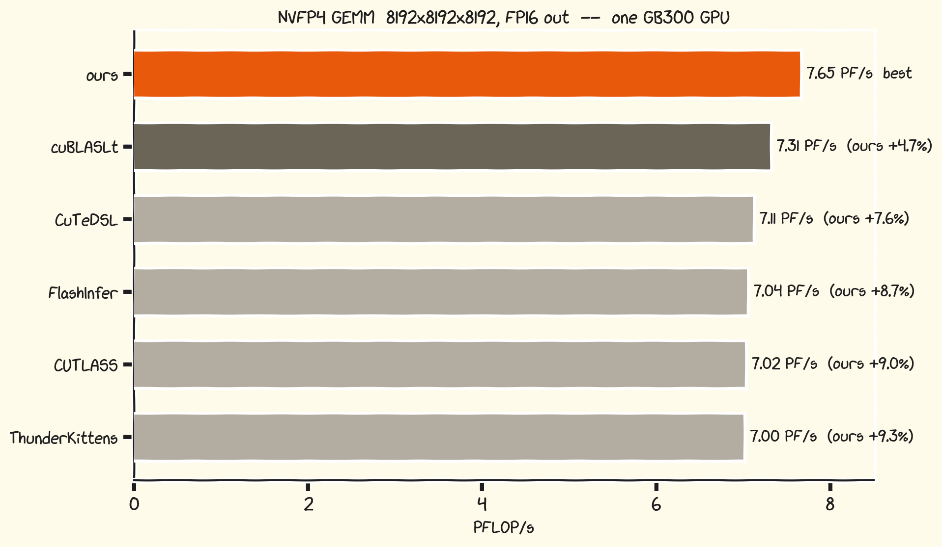
Here are our final numbers on a GB300 node with CUDA 13.1:
All code is available in Github here.
We will first build an NVFP4 GEMM from scratch for GB300, as always in plain CUDA and inline PTX, with no framework dependency. We will focus first on the classic 8192 x 8192 x 8192 shape, outperforming cuBLAS by 4.7%. We also show results on some other shapes.
We choose NVFP4 because it presents more challenges than other dtypes. As tensor-core instructions get faster, the rest of the pipeline struggles to keep them fed. That’s where we can showcase the most extreme GPU performance tricks. Additionally, entire kernels are 100% generated by Claude(more on this later).
I hope this motivates people to own their kernels, and not treat them as blackboxes. Everything is just yet another piece of code.
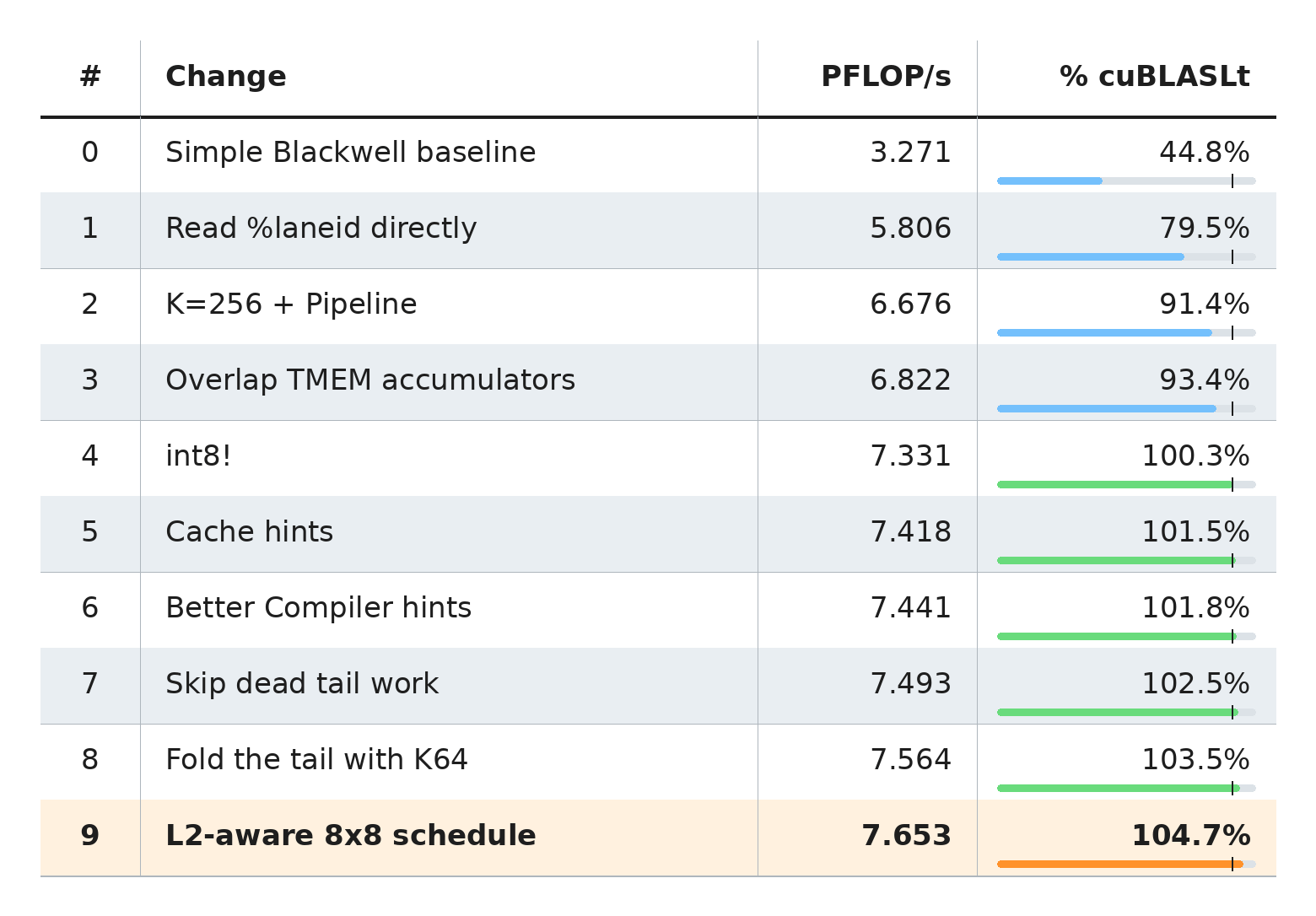
The Optimization Ladder
What is NVFP4?
NVFP4 means NVIDIA’s floating point in 4 bits. Each matrix value is stored in the 4-bit E2M1 format:
1 sign bit
2 exponent bits
1 mantissa bit
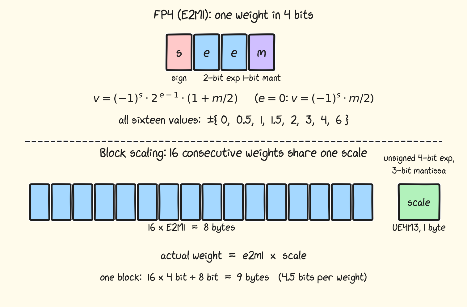
The representable magnitudes are 0, 0.5, 1, 1.5, 2, 3, 4, and 6. That range is too small for a useful tensor by itself, so every group of 16 values along K shares an 8-bit UE4M3 scale factor (multiply each value by this number to get the dequantized value).
This makes the effective storage cost 4.5 bits per value.
It’s pretty simple to get these from the original BF16 values: take the maximum absolute value in each 16-value block and divide it by 6 (E2M1’s largest value) - this becomes the scale. Then normalize each value by this scale to fit into FP4. This ensures we set the scale so that each value is at most 6.
Blackwell can consume this format directly. The tcgen05.mma instruction reads E2M1 values and their scale factors, applies the scales inside the tensor core, and accumulates into FP32. There is no separate dequantization loop.
Building a Working Blackwell Kernel
A basic Blackwell kernel looks very different from Hopper. Blackwell tensor cores are more “asynchronous” than Hopper tensor cores. Hopper threads need to allocate several registers to hold the output of tensor-core operations. The threads are free to do something else while the operation runs, but the lack of spare registers makes it hard to actually do anything useful.
Blackwell moves those accumulators into a separate on-SM memory, Tensor Memory (TMEM), leaving the CUDA threads free to do other work.
I will not re-teach every Blackwell instruction here. The posts linked above already do that well. Instead, I will first quickly develop a Blackwell-style prototype with several important details already in place, while still leaving a large gap to cuBLAS. This section will read more like a speedrun over these basic techniques, and then we can have more fun.
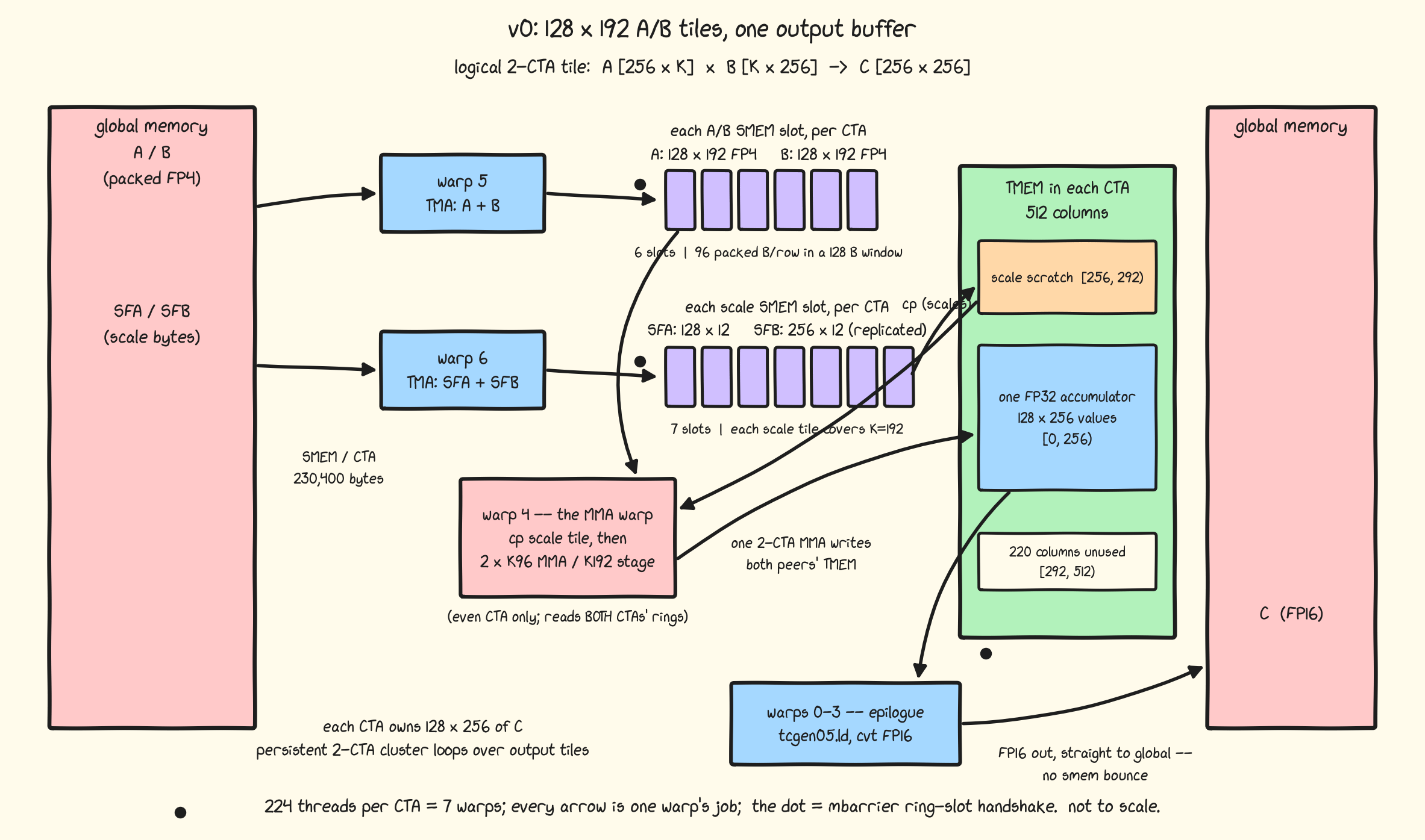
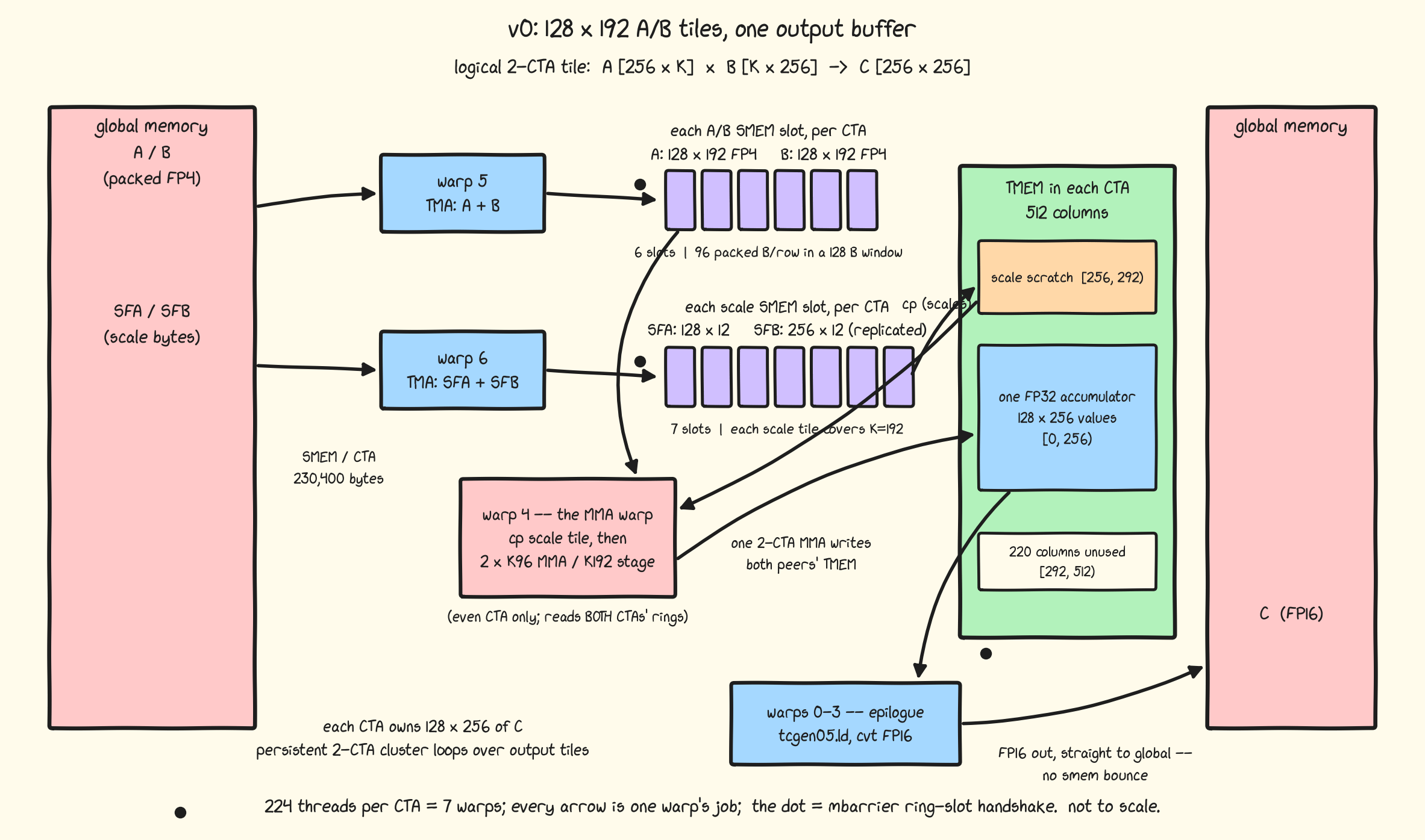
Here is how I like to visualize kernels: as a data flow showing where each operand lives and how it moves through HBM, shared memory, tensor cores, tensor memory, and registers.
Seven warps, four roles
Each CTA has 224 threads, or seven warps. Warps 5 and 6 load data into shared memory queues, warp 4 consumes them and issues MMAs, and warps 0-3 store the MMA result into global memory.
Warps  Role
-----  --------------------------------------------------------------------------------
0-3    Read FP32 accumulators from TMEM, convert to FP16, and store
4      Copy scale factors from SMEM to TMEM and issue every MMA (which outputs to TMEM)
5      Load A and B into shared memory with TMA
6      Load A and B scale factors into shared memory with TMA
As on Hopper, each warp synchronizes with others using mbarrier and exchanges data using either Shared Memory or Tensor Memory (new).
The K=96 MMA
GB300 introduces a bigger MMA shape than the GB200 version. K = 64 --> 96, which is 50% larger but takes the same number of cycles (at the largest shape).
M    N    K   Cycles  Performance at 2 GHz
---  ---  --  ------  --------------------
256  128  64  64      10.0 PFLOP/s
256  128  96  78      12.3 PFLOP/s
256  256  64  128     10.0 PFLOP/s
256  256  96  128     15.0 PFLOP/s
So naturally, we need to use the largest possible tile size, that is 256 x 256.
Two CTAs per output tile
Blackwell has a specific way to do 2-CTA tensor core instructions, natively supporting larger tile sizes (compared to Hopper, where we just multicast operands). This lets 2 CTAs running on 2 SMs in the same cluster coordinate and run a larger tensor core operation. This increases our tile size from 128 x N to 256 x N.
tcgen05.mma.cta_group::2.kind::mxf4nvf4.block_scale.scale_vec::4X
  [%0], %1, %2, %3, [%5], [%6], acc;
In this mode, the shared memory required to read A and B is split across both CTAs, and at the end the output is also split in half across the two CTAs:
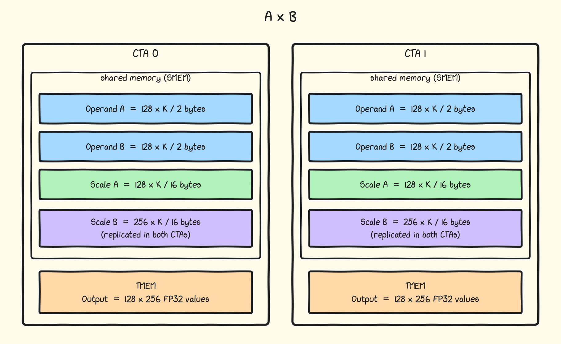
Note that every load is equally sharded across the 2 SMs - but the scale factors for the B matrix need to be replicated (for faster hardware access, I presume).
Here is how it looks: Both CTAs run the same two producer roles and walk K in 192-value stages (packing two K=96 MMAs, which we will get to next):
// Runs in both CTAs.
int m_cta = tile_m + 128 * cta_rank;
int n_cta = tile_n + 128 * cta_rank;

if (warp_id == 5 && (threadIdx.x % 32) == 0) {
    for (int k = 0; k < K; k += 192) {
        wait(ab_free[ab_slot]);
        if (cta_rank == 0)
            expect_tx(ab_ready[ab_slot],
                      2 * (128 * 96 + 128 * 96)); // 2 CTAs x (A + B)
        tma_load(a_smem[ab_slot], (m_cta, k)); // packed: 128 x 192
        tma_load(b_smem[ab_slot], (n_cta, k)); // packed: 128 x 192
        ab_slot = (ab_slot + 1) % 6;
    }
}

if (warp_id == 6 && (threadIdx.x % 32) == 0) {
    for (int k = 0; k < K; k += 192) {
        wait(sf_free[sf_slot]);
        if (cta_rank == 0)
            expect_tx(sf_ready[sf_slot],
                      2 * (128 * 12 + 256 * 12)); // 2 CTAs x (SFA + SFB)
        tma_load_4d(sfa_smem[sf_slot], (m_cta, k)); // logical: 128 x 12 scales
        tma_load_4d_multicast(
                    sfb_smem[sf_slot],
                    (tile_n, k, cta_rank),
                    both_ctas);                  // logical half: 128 x 12
        sf_slot = (sf_slot + 1) % 7;
    }
}
Note: For Scale B, each CTA loads half of the 3,072-byte slot and multicasts it to its peer. That is 0.3% faster than making each CTA load the whole slot.
NVFP4 packs two values per byte, so each 128 x 192 FP4 tile is a128 x 96-byte TMA load. The scale factors are loaded in groups of 128 x 12, 12 elements per row. Let’s see why 12 makes sense next - and what’s up with the 4d TMA.
Scale factors need special handling
The MMA reads A and B through SMEM descriptors, but its scale factors have
to live in TMEM. This instruction copies them there:
tcgen05.cp.cta_group::2.32x128b.warpx4 [%0], %1;The HBM buffer uses the same standard VEC16 scale layout as cuBLASLt; there is
no kernel-specific repack. We describe that buffer to TMA as four dimensions:
outer block, a group of four K scales, the scale inside that group, and 128
contiguous row bytes. A box of 3 x 4 x 128 bytes therefore lands as the
logical 128 x 12 SMEM tile expected by 32x128b.warpx4. For more details on
this special swizzling, I will defer to gau-nernst’s tcgen05 blog - it does not directly influence our algorithm.
The more important arithmetic for us is that one K=96 MMA consumes six scale bytes per row. If we stage two MMAs at a time, and tcgen05.cp moves 512-byte tiles:
A scales: 128 rows x 6 x 2 bytes = 1,536 bytes = 3 cp tiles
B scales: 256 rows x 6 x 2 bytes = 3,072 bytes = 6 cp tiles
2 MMAs are grouped because we want to fully utilize the 512-byte copy range of tcgen05.cp - which is an optimal choice.
The K=192 TMA tile size comes directly from this arithmetic.
The resulting three SFA copies and six SFB copies occupy exactly 36 TMEM columns.
Warp 4 consumes one scale slot and one A/B slot together, and just walks K in 192-value stages:
if (cta_rank == 0 && warp_id == 4 &&
    (threadIdx.x % 32) == 0) {
    wait(acc_free, d_parity);

    for (int k = 0; k < K; k += 192) {
        wait(sf_ready[sf_slot]);
        copy_3_sfa_and_6_sfb_tiles_to_tmem(sf_slot);
        commit(sf_free[sf_slot]);

        wait(ab_ready[ab_slot]);
        mma_k96(k);
        mma_k96(k + 96);
        commit(ab_free[ab_slot]);

        sf_slot = (sf_slot + 1) % 7;
        ab_slot = (ab_slot + 1) % 6;
    }
    commit_multicast(acc_ready, both_ctas);
}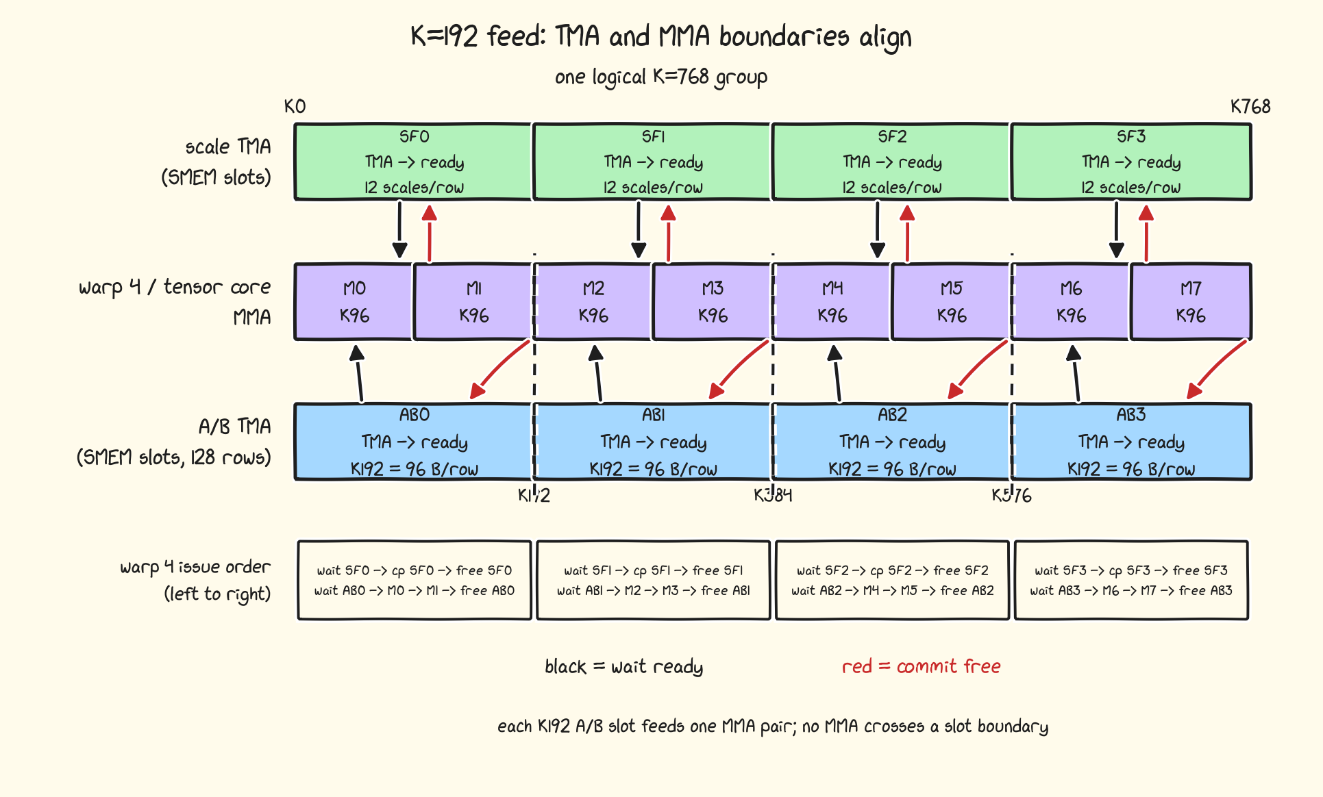
From the diagram, the choices of tile sizes make sense - everything aligns pretty well.
A few interesting points to note:
Both
commitcalls are asynchronoustcgen05.commitoperations carrying an mbarrier arrival. They don’t happen immediately, but after the correspondingcpormmacall finishes.Note that a single warp issues both
tcgen05.cpandtcgen05.mma. Under PTX’stcgen05memory-consistency rules,tcgen05.cpintotcgen05.mmais explicitly pipelined. We don’t have to wait formmato finish before issuing anothercpthat would overwrite the scale factors in the same TMEM space. This is safe because thecommitaftermmaimplicitly performstcgen05.fence::before_thread_sync, ordering both MMAs before the following copy. This establishes an ordering that is followed by the tensor cores.
Reading from TMEM
With a 256 x 256 tile, each CTA receives a 128 x 256 FP32 output in TMEM, or 256 columns. We use one accumulator buffer at columns [0, 256) and one reusable 36-column scale region at [256, 292). The other 220 of TMEM’s 512 columns are unused (but will come in handy later).
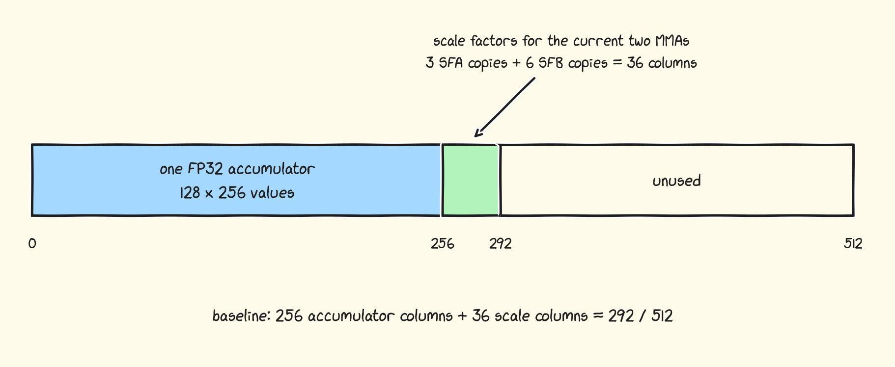
Warps 0-3 handle the drain. Each warp owns 32 rows, while the two CTAs together contribute arrivals to acc_free after the whole tile has been loaded from TMEM to registers:
if (warp_id < 4) {
    wait(acc_ready);

    for (int band = 0; band < 8; ++band) {
        float acc_regs[32]; // 32 registers per lane
        tmem_load_x32(tmem_base + 32 * band, acc_regs);

        if (band == 7) {
            wait_for_tmem_loads();
            arrive(acc_free);
        }
        store_fp16(acc_regs, output_row, 32 * band);
    }
}
The important loop is therefore not one producer followed by one consumer. It is three independent handshakes running at once: TMA fills the SMEM rings, some warp moves scales and launches MMAs, and the epilogue returns the accumulator only after loading all of it out of TMEM.
If this felt too overwhelming, it makes sense to look at this data flow diagram again:
Optimization 1: Read %laneid Directly
Several warp roles need exactly one thread in a warp. For example, warp 4 looks like this:
if (cta_rank == 0 && warp_id == 4 && threadIdx.x % 32 == 0) {
    run_mma_role();
}
It feels very natural to write this. HOWEVER, if you switch to reading the %laneid special register directly, it is a whopping 77.5% faster (nani?!?)
__device__ __forceinline__ uint32_t lane_id() {
    uint32_t lane;
    asm("mov.u32 %0, %%laneid;" : "=r"(lane));
    return lane;
}
if (cta_rank == 0 && warp_id == 4 && lane_id() == 0) {
    run_mma_role();
}
The two conditions are mathematically identical, but ptxas does not compile them the same way. I made the same substitution at all five single-lane sites. It moves the kernel from 3.271 to 5.806 PFLOP/s!
To understand the gap, it helps to know about uniform registers. A normal
GPU register holds a separate value for each of the 32 lanes in a warp. A
uniform register holds one value for the whole warp, and the uniform
datapath can calculate with it once instead of repeating the same work in
all 32 lanes.
Our SMEM descriptors, TMEM addresses, barrier addresses, and loop state are
all warp-uniform. Ideally ptxas keeps them on that cheaper path. Starting
the check from threadIdx.x, a per-thread value, makes the compiler lose some of that proof (though it could be better!).
It then inserts R2UR SASS instructions to copy values from regular registers into uniform registers, plus instructions that track which lanes are active. The direct %laneid form is recognized much better: this version has 135 fewer R2UR instructions and the SASS is 848 lines shorter.
Optimization 2: K=256 + Pipeline
So far each A/B TMA tile covers a 128 x 192 shape. Our next goal is to increase it to 128 x 256.
192 fits well with K=96. But the TMA operation can be more efficient if we make the inner dimension 128 bytes wide. However it makes tiles uneven and needs very careful barrier surgery:
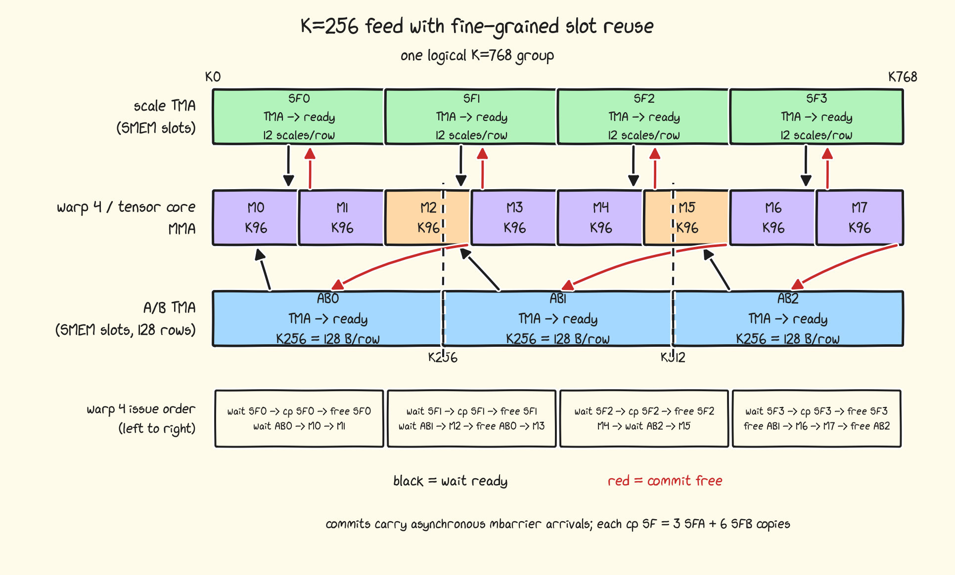
This diagram looks a bit more complicated than our last one. But the core flow is simple: wait for the things you need, and free them as soon as you are done.
MMA waits for both A/B and scale factors A/B, and as soon as MMA is done, it can free the respective buffers. But the different buffer sizes mean the ordering has to be manually staged. Since we have a fixed K=768, we can manually unroll everything and release/queue requests as soon as possible without any overhead.
The diagram is the best explanation of barrier details - so I’d recommend going through it if you’re interested.
When MMA5 is done, for example, we can free AB1 right away. However, we choose to issue SF3 first. It turns out to be important that we issue the
cpfirst - it breaks the serialization ofcpandmma. A natural question is: why not use another warp to do thecpand add more mbarriers? In many cases, we don’t have an extra warp (due to CLC), and mbarriers have a slight cost as well in the FP4 regime.
Another interesting fact is that the TMA and MMA partitions no longer have the same boundaries. So MMA2 has to read parts of both AB0 and AB1.
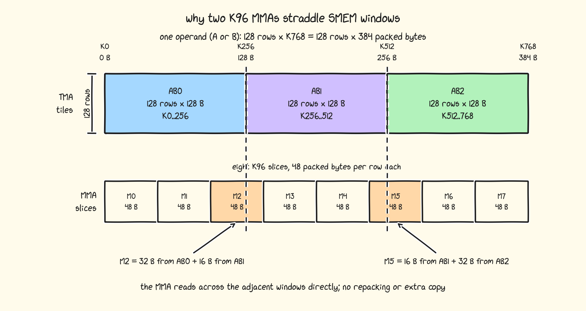
The top row is how TMA writes the operand; the bottom row is how the tensor core reads the exact same bytes. The two orange MMAs simply cross into the next 128-byte window.
PTX has a descriptor mode specifically for this case: absolute address mode for a 48-byte K dimension. This can be specified in the instruction descriptor for the tcgen05.mma call.
  desc =
      encode(AB0 + 96)       // first 32 B begin in AB0
    | encode(AB1) << 16      // final 16 B comes from AB1
    | FIXED_K96_SW128_BITS;
This gets us from 5.806 to 6.676 PFLOP/s, 15.0% faster!
Shared-memory accounting
  1,024 B          barrier header + padding
6 x 16,384 B       A ring
6 x 16,384 B       B ring
7 x  1,536 B       A scale-factor ring
      512 B        alignment padding
7 x  3,072 B       B scale-factor ring
----------------
230,400 B          total per SM
Each CTA uses 230,400 of 232,448 available bytes: 99.1%.
Six A/B stages and seven scale stages keep TMA ahead of the MMA warp.
Dropping one A/B stage costs 12%; dropping one scale stage costs 1.2%.
Optimization 3: Overlap Two Accumulator Buffers
Our loads and MMA are now pretty well parallelized. But the MMA warp still waits for the epilogue to empty its TMEM output buffer before starting work on the next tile. Ideally we want to store 2 of these, so the tensor core thread doesn’t wait for the consumer warps to read and free it - and immediately starts the next MMA loop.
But if we do this, there is no space left for the scale factors (they need to be in
TMEM as well):
2 x 256 accumulator columns + 36 scale columns = 548 > 512The solution is to overlap the two output tiles by 36 columns (548 - 512). So
the MMA only has to wait for the consumer to drain the overlapping edge
instead of all 256 columns of the old buffer. We delay the synchronization
instead of completely removing it.
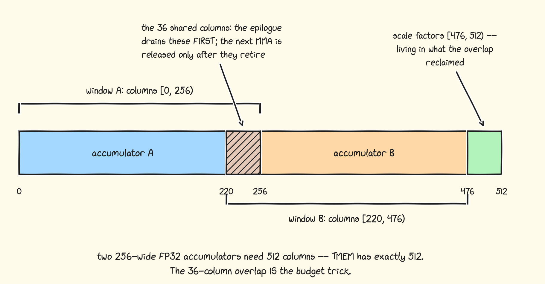
Warps 0-3 handle this drain (one thread per row).
if (warp_id < 4) {
    wait(acc_ready);

    for (int i = 0; i < 8; ++i) {
        int band = (d_parity == 0) ? 7 - i : i;  // overlap first
        float out[32];
        tmem_load_x32(tmem_base + 32 * band, out);

        if (i == 1) {
            wait_for_tmem_loads();
            arrive(acc_free);
        }
        store_fp16(out, output_row, 32 * band);
    }
}
Note that the loads from TMEM to registers are only 32 columns wide. We can do more if needed, but it turns out this is enough to get the best performance. As a result, we only use 32 registers, which is pretty cheap and does not need the custom register allocation that Hopper required.
One thing that didn’t work out: We only need to signal
acc_freeafter reading 36 columns, but we do so after 64 columns. I tried to fully unroll loads into multiple sizes and release earlier at 36 columns, but it was 0.5% slower. So I kept this simpler version.
It’s helpful to look at the complete flow one last time. The output tile is still 256 x 256, but A/B stages fill their full 128-byte SMEM windows and TMEM now carries two output tiles at once:
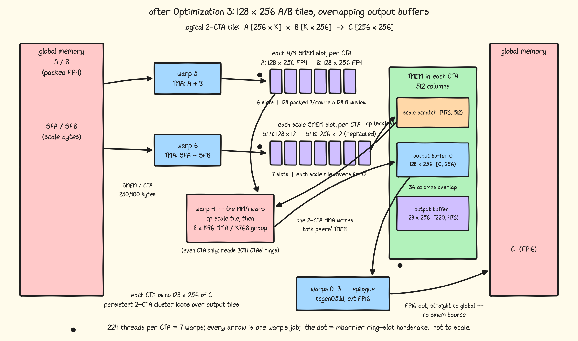
This moves the kernel from 6.676 to 6.822 PFLOP/s, a 2.2% gain.
Optimization 4: int8!
At this point, we have moved from optimizations to micro-optimizations.
Starting with Blackwell, CUDA has support for 256-bit loads/stores - basically int4 now has a more powerful variant: int8. It’s actually called longlong4_32a. I prefer to use the PTX instruction directly:
"st.global.v8.b32 [%0], "
"{%1, %2, %3, %4, %5, %6, %7, %8};"
This moves the kernel from 6.822 to 7.331 PFLOP/s, a 7.5% gain - and we are already at 100.3% of cuBLAS!
Optimization 5: Cache Hints
Store width is only half of the instruction. The same store also carries
the output cache policy:
st.global.L1::no_allocate.L2::evict_first.v8.b32 [%0],
{%1, %2, %3, %4, %5, %6, %7, %8};
The output is written once and is not read again by this kernel.L1::no_allocate prevents those stores from allocating lines in L1, where
they would compete with the input pipeline. The data still passes through
L2, so L2::evict_first makes those lines the first eviction candidates
and leaves more room for reusable inputs.
This moves us from 7.331 to 7.418 PFLOP/s, a 1.2% step.
Optimization 6: Better compiler hints
- __global__ __cluster_dims__(2, 1, 1) __launch_bounds__(224, 1) kernel(...) {}This is how we have been launching the kernel. Cluster dims tell the compiler the cluster size, and launch bounds tell it the kernel will use at most 224 threads. However, there is a new performance hint in town:
+ __global__ __block_size__((224, 1, 1)) __cluster_dims__(2, 1, 1)
+   __launch_bounds__(224, 1) kernel(...) {}
__block_size__(224) says exactly 224 threads. This is labeled as the reqntid performance directive in the PTX guide.
When ptxas cannot prove a complete warp reaches each collective, it inserts convergence guards. However, the new performance directive solves this and reduces BSSY/BSYNC SASS instruction pairs and register usage from 62 to 52!
This is only a 0.3% throughput step in the rebuilt chain, from 7.418 to
7.441 PFLOP/s, but the generated-code cleanup is real.
Optimization 7: Skip the Dead Tail
The mainloop naturally repeats every K=768: three K=256 A/B stages, four
K=192 scale stages, and eight K=96 MMAs all line up. K=8192 leaves a
512-element tail after ten full groups. The baseline still runs one complete
tail group, so its last eight MMAs look like this:
MMA 0  1  2  3  4       5             6  7
    96 96 96 96 96   32 real + 64 zero   all zero
This is not host-side extra padding. TMA’s out-of-bounds fill supplies the
zeros, but the tensor core still spends time multiplying them.
To fix this, I kept the fast K=768 loop untouched and added one explicit tail group:
int full_groups = K / 768;
int remainder = K % 768;

run_k768_groups(full_groups);
if (remainder != 0) {
    int tail_mmas = ceil_div(remainder, 96);
    run_tail_group(tail_mmas);
}
Other warps skip the same ring entries and barriers; otherwise it’s very easy to create a deadlock here.
The K=8192 kernel now computes K=8256 rather than K=8448. That moves the perf from 7.441 to 7.493 PFLOP/s, a 0.7% gain.
Optimization 8: Fold the Tail with K64
The exact feed no longer pads to K=768, but its last tensor-core instruction is still K=96. For K=8192, we can be exact by mixing K96 and K64 instructions:
Full-group tail:    11 x 768                         = 8448
K96-only tail:     10 x 768 + 6 x 96                 = 8256
folded K64 tail:   10 x 768 + 4 x 96 + 2 x 64        = 8192
The specialization moves the release audit from 7.493 to 7.564 PFLOP/s,
another 0.9%.
At this point, we are directly handrolling optimizations directly for the 8192 x 8192 x 8192 shape. Now, let’s move on to handrolling for the GPU instead.
Hardware aware Scheduling
Our baseline scheduler walks the output grid in a simple row-major order. This gets very good L2 cache hits for one of the matrices, but none for other. In my previous H100 worklog, we grouped nearby tiles into pockets to improve L2 reuse for both matrices:
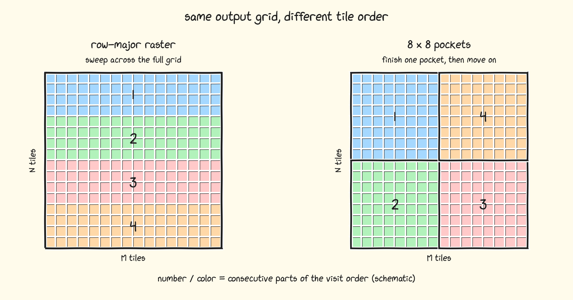
Tiles in same color run at the same time across all available SMs. This means they enjoy the cache benefits of reading same parts of A/B matrices they require.
Let’s see how this idea performs:
Tile order   PFLOP/s
-----------  -------
Row major    7.570
8x8 pockets  7.508
Our theory is sound, but it’s not very clear why this performs badly. To tackle this, we first need to understand some hidden hardware details about L2 cache. We will formulate a theory, and use it to make the 8x8 pockets work in practice.
The L2 is Actually Two Caches
GB300 is two dies in one package. Its 152 SMs split into two groups, and each group sits next to roughly half of the 128 MB L2.
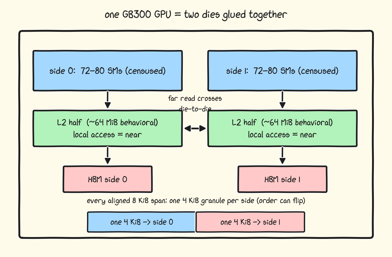
There are two different meanings of “side” here:
Every physical address has a home side, selected by an address hash.
Every SM has a near side, determined by which die contains that SM.
These labels need not match. If an SM on side 0 asks for a line homed on side 1, the cold read crosses the die-to-die link.
Requester relative to the line's home side  atomicAdd Latency
------------------------------------------  -----------------
Near                                        148 ns
Far                                         344 ns
To expose the hop, I used a dependent atomicAdd chain: each returned value
feeds the next address, leaving no memory-level parallelism to hide the
latency. A remote round trip is ~2.3x slower.
However, this does not directly make GEMM faster because our TMA queue keeps many requests in flight and hides the hop pretty well. A more interesting fact is how this directly influences effective L2 cache size.
How is the L2 cache split
The partitioned L2 cache idea is not well-known, but there are enough crumbs on the internet to piece it together. NVIDIA first described it in the A100 whitepaper,
it was microbenchmarked by Citadel, I briefly mentioned this in my last blog and Aroun actually did the address calculation for Blackwell in QuickRunCUDA - which I have ported.
The address mapping is as follows:
side = parity(physical_address & 0x1EF000) ^ slab_phase;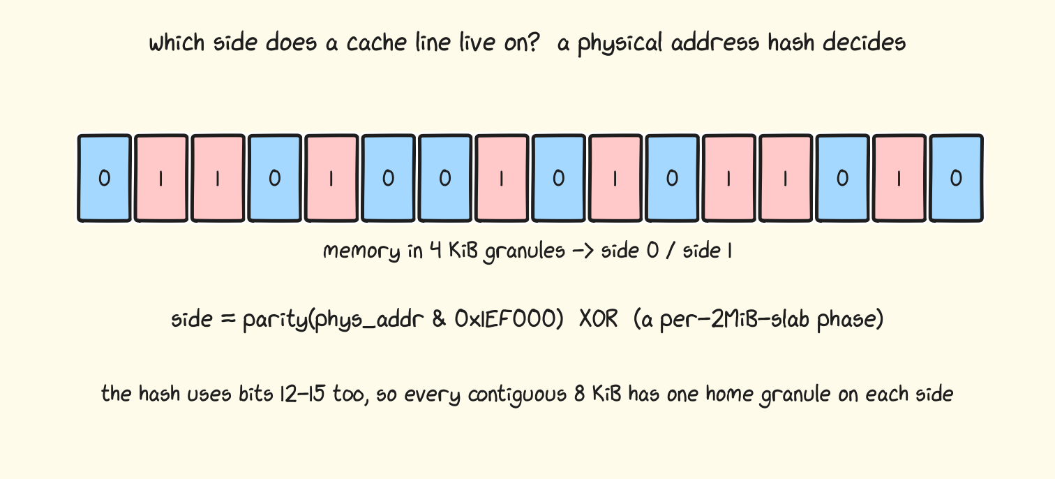
What it says is that every 4 KB memory segment will fall entirely on side 0 or side 1. Every aligned 8 KB span also contains one segment for each side. This mapping is deterministic within a 2MB slab, but different 2MB slabs may have complementary mappings(that is the near and far sides are flipped).
For GEMM, we don’t need to dive deep into exactly which mapping goes where, we just need to group SMs into 2 sets so they can exclusively use their “own” L2 cache space. This grouping can be found by checking memory latency on same address.
Not all GPUs are born equal
First, one important detail: with 152 SMs, you might expect every GPU to
split 76:76 for the L2 sides. Some do, but the split ratio is not fixed. These are the ratios I have seen:
SMs on side 0 / side 1  Two-CTA clusters
----------------------  ----------------
76 / 76                 38 / 38
72 / 80                 36 / 40
74 / 78                 37 / 39
2 SMs in a cluster always land on same side, but its not an even split. So every GPU is slightly different, and you may even see different “effective” L2 cache sizes in them. Power issues are not the only ones to blame for variance in GPU performance!
Optimization 9: 8x8, but L2-Aware
The failed 8x8 experiment tells us exactly what is missing. A local order can get larger L2 cache hits, but without coordinating they may just thrash each other. There are 2 orthogonal factors:
Ownership decides where reuse happens. One SM side gets every repeat
read of an A tile.
Order decides when reuse happens. Within each side, 8x8 pockets keep
the next use nearby.
For one output tile,
C[m,n] = sum_k A[m,k] * B[n,k]Holding m fixed reuses A[m,:] and SFA across N. I therefore assign each
output row m to one requester side. B and SFB stay shared because each N
tile is needed by M rows on both sides.
This does not automatically place A in one physical L2 half. Every A row is still about 50/50 by home address, so some first touches cross the link. What changes is who comes back: only clusters from the row’s owner side reread it. A cold line may be remote, but its later N reuse stays with one requester population instead of building useful residency in both halves.
At 8192 cubed, the output grid is 32 x 32 tiles. On CPU side, we prcompute the exact number of loop trips for each cluster, assigns whole M rows to two side pools, then walks each pool in 8x8 pockets. We store this schedule in a route table where each SM can reference to know which tile to compute. This table is only a few KB, with one entry per 256x 256 tile.
The wins
Strategy                    PFLOP/s
--------------------------  -------
Row-major                   7.570
8x8 pockets / Hilbert       7.508
8x8 pockets + L2 ownership  7.646
Something for every shape
Every shape can works best with a slightly different schedule.
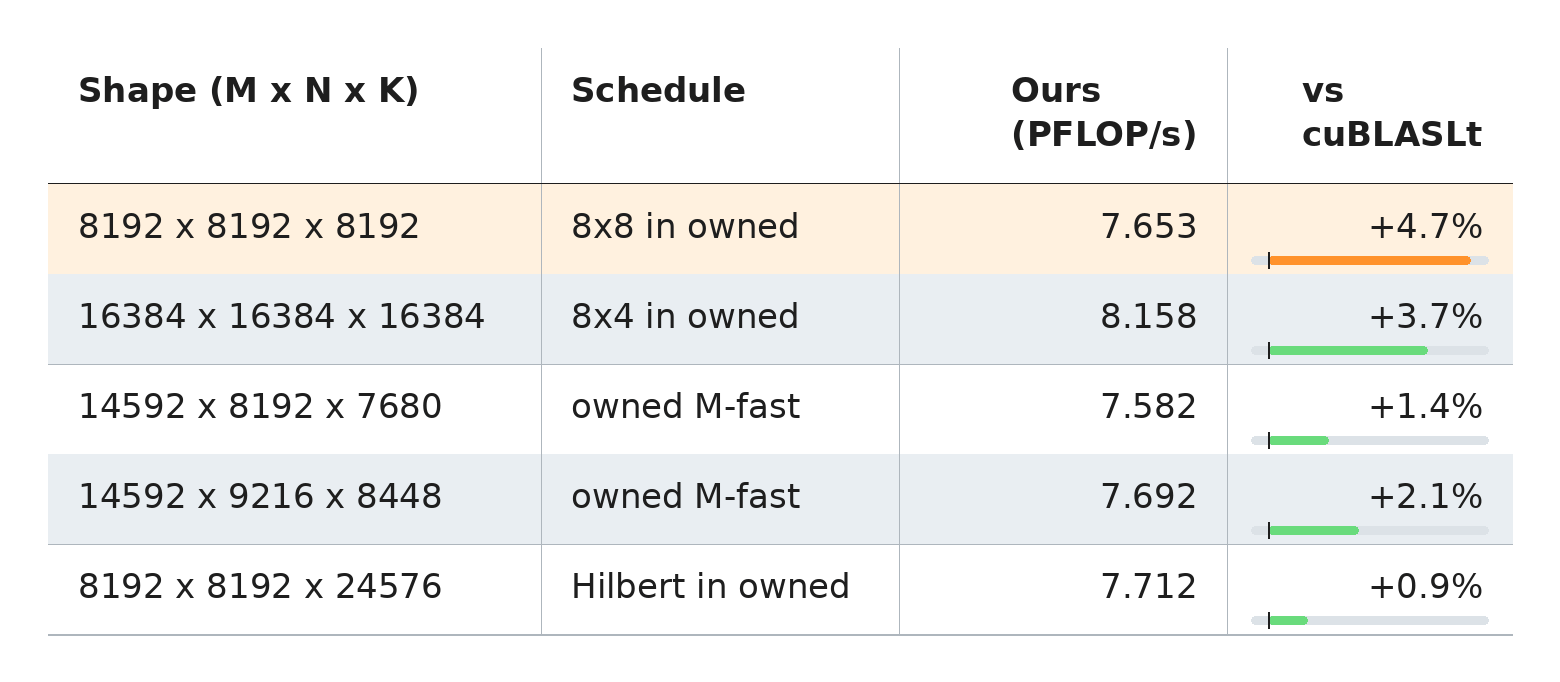
This doesn’t mean we are faster than cuBLAS at every shape. (In fact, I did not beat it on several shapes with this code). But it highlights the possibility to “Compile” your kernels for every shape!
One last micro-optimization
A small detour, we can use redux.sync instruction to hint the compiler that the schedule information can also be stored in a uniform register.
uint32_t tile = route_table[table_offset + t];
uint32_t uniform_tile;
asm("redux.sync.min.u32 %0, %1, 0xffffffff;"
    : "=r"(uniform_tile) : "r"(tile));
The route decode and address arithmetic can then stay on the uniform path which is always better. This has negligible effect on performance but keeps the SASS clean. I only add this because it was incredibly hard to find, I wish PTX had better compiler hints baked into it.
Benchmarking Methodology
for (...) kernel(A, B, C);Rotate inputs. Every launch uses a different copy of A and B, so the kernel cannot see its own previous inputs in L2.
Multiple rounds. Our kernel and cuBLASLt alternate for five rounds. We also rotate which one runs first each time. In each round, we launch 25 kernels back to back with rotated inputs and take their mean.
Cool down GPU. Each timed arm gets at least eight seconds to cool down. The goal is for GPU to reach a cooled-down state before next round. If it doesn’t(the idle GPU clock has not returned back to original state), we keep sleeping and polling till it does.
There is no single right way to benchmark kernels. With power bound kernels, numbers always vary a little. Just make a way you can be confident of incremental improvements by having less variance in each measurement. Here I will show 4 ways to benchmark our kernel, all showing different wins over cuBLAS:
Method                       Ours (PFLOP/s)  cuBLASLt (PFLOP/s)  Ratio
---------------------------  --------------  ------------------  -------
Current protocol             7.653           7.307               1.0473x
Triton-style with L2 clears  7.179           6.711               1.0698x
Clock locked to 1305 MHz     6.734           6.245               1.0783x
Sustained 60-second blocks   6.424           6.181               1.0392x
The current row is the protocol used throughout this post. The sustained test gives the smallest margin, while locking the clock exposes the largest per-cycle difference. I use the current protocol for the headline because I feel its more representative of real workloads.
Conclusion
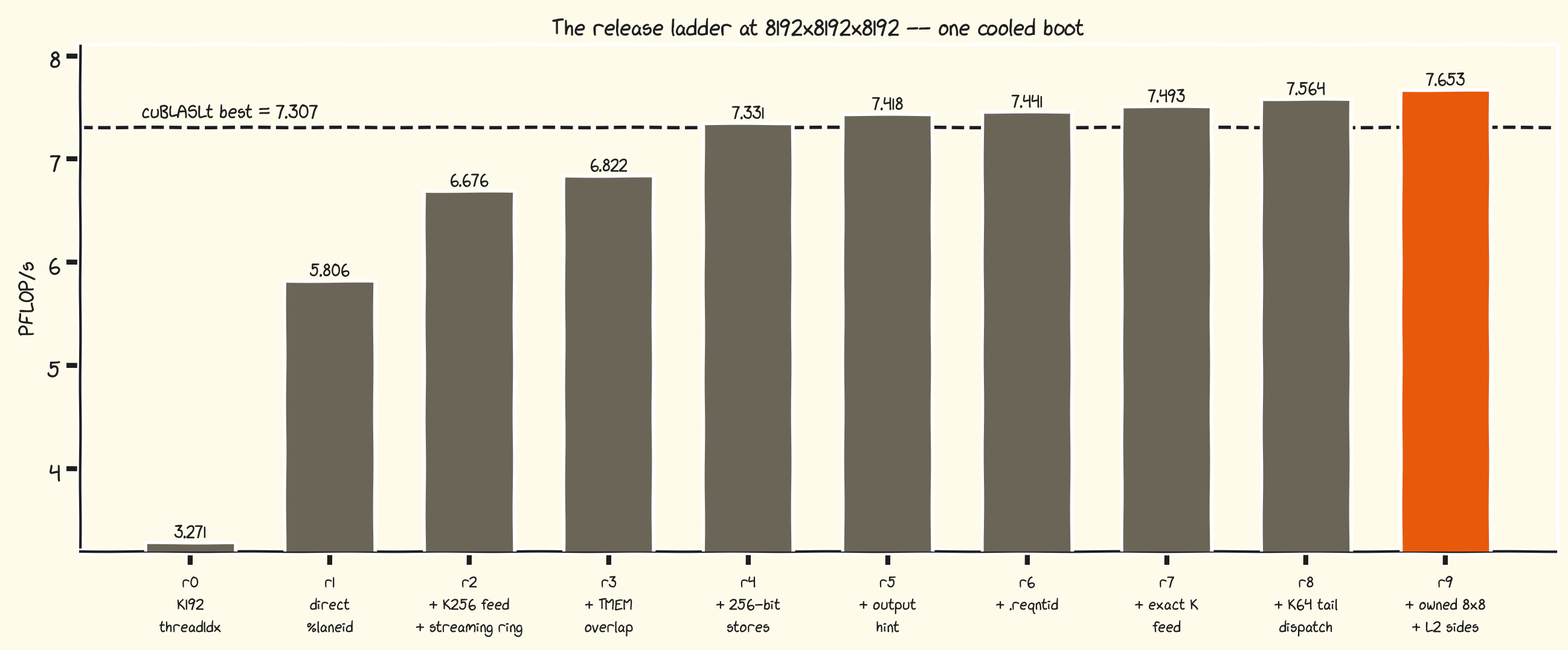
We wrote a NVFP4 matrix multiplication kernel from scratch, reaching 4.7% over cuBLAS - best baseline that I know of. Perhaps the most interesting optimization is the last one as it utilizes internal details of L2 cache in Nvidia GPUs to develop a faster scheduling algorithm.
AMD GPUs also have this quirk - but they are very loud about it and often co-design with that in mind.
As much as I’d like to do more posts, the age of getting nerdsniped over algorithms is over. In future, I will be sharing more on how to best use AI agents for GPU peformance.
Resources
Claude Code
gau-nernst’stcgen05notesademeure’s QuickRunCUDA side aware experiment
Daniel’s MXFP8 blog
Outperforming cuBLAS on BF16 by Paul Chan
Outperforming cuBLAS by Ali and Modular team